A generalised Newton iteration scheme

As another practical example of the use of the template file approach, consider writing a general program for solving a system of equations of the form:  

$${\bf f}({\bf x})={\bf 0}$$ (2)

using Newton's method [32]. A bold typeface is again used to denote a vector.

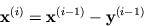
The system of iterates can be written as:  

$${\bf x}^{(i)} = {\bf x}^{(i-1)} - ({J^{(i-1)}})^{-1} \, {\bf f}^{(i-1)} \quad , \quad i = 1,\ldots,itmax$$ (3)

where $J = {\partial {\bf f}({\bf x}) \over {\partial {\bf x}}}$ denotes the Jacobian matrix and ${\bf x}^0$ is a given set of initial values used to start the iteration process. (J^k)^-1 denotes the inverse of J^(k) and the superscript k denotes evaluation at iterate ${\bf x}={\bf x}^{(k)}$. The iterative process is continued until some stopping criteria are satisfied at iteration itmax. When the system to be solved is scalar valued, (J^k)^-1 is simply the reciprocal of J^k. For practical implementation, (3) is rewritten at each iteration as:  

$${\bf x}^{(i)} ={\bf x}^{(i-1)} - {\bf y}^{(i-1)}$$ (4)

where ${\bf y}^{(i-1)}$ satisfies  

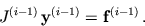$$J^{(i-1)} \, {\bf y}^{(i-1)} = {\bf f}^{(i-1)} \,.$$ (5)

The linear system (5) is typically solved using LU decomposition of the Jacobian matrix at each iteration. The value of ${\bf y}^{(i-1)}$ thus obtained is substituted into (4) to obtain ${\bf x}^{(i-1)}$.